Manual

Global Nonlinear Least-Squares Equilibrium Analysis:

The UltraScan global nonlinear least squares fitting program for equilibrium data provides a number of predefined models, each is discussed in further detail below. Each model has a global model number, which is used in default naming conventions for result files, Monte Carlo analyses and as a model descriptor across different methods. The model number is indicated in each description:

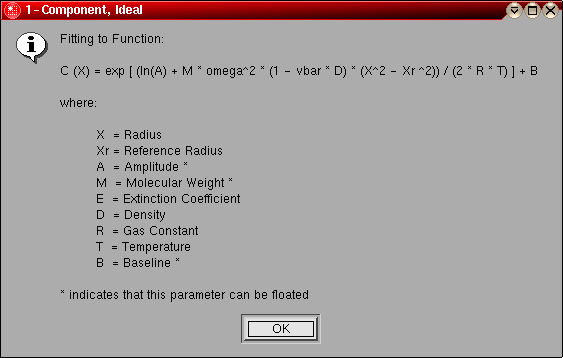
1. 1-Component, Ideal: This model can be used for a pure, single component system that behaves hydrodynamically ideal. This model should be used first, if model fits well, the system is homogeneous and doesn't self-associate. The following parameters are fitted:
   • A single molecular weight (global)
   • The log of the amplitude of the molecular weight term for each included scan (local)
   • The baseline for each included scan (local)

   The model number for this model is "0".

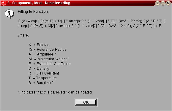
2. 2-Component, Ideal, Noninteracting: This model can be used for for a system of two components that are not interacting, and behaving hydrodynamically ideal. After fitting this model, and a good fit was obtained, it is a good idea to compare the ratios of the integrals between scans run under different conditions.

   If the ratios are roughly unchanged from scan to scan (by an order of magnitude), there is a good chance that the system is truly noninteracting and two different components are in the system. If the ratios change in the direction of larger amounts for the larger component with increasing concentration and speed, the model should be fitted with a self-associating model, since the molecular weight average changes with concentration distribution, and a concentration-dependent self-association is most likely present. The following parameters are fitted:

   • The molecular weight for component 1 (global)
   • The molecular weight for component 2 (global)
   • The log of the amplitude of molecular weight term 1 for each included scan (local)
   • The log of the amplitude of molecular weight term 2 for each included scan (local)
   • The baseline for each included scan (local)

   The model number for this model is "1".

3. 3-Component, Ideal, Noninteracting: This model can be used for for a system of three components that are not interacting, and behaving hydrodynamically ideal. After fitting this model, and a good fit was obtained, it is a good idea to compare the ratios of the integrals between scans run under different conditions. If the ratios are roughly unchanged from scan to scan (by an order of magnitude), there is a good chance that the system is truly noninteracting and three different components are in the system.

   If the ratios change in the direction of larger amounts for the larger components with increasing concentration and speed, the model should be fitted with a self-associating model, since the molecular weight average changes with concentration distribution, and a concentration-dependent self-association is most likely present.

   Because this model has a large number of degrees of freedom, this model should only be used for cases where all other models fail to describe the system. Rarely do equilibrium scans contain enough information to quantitatively describe a three component system with all of its parameters floated. However, if you do know the molecular weight of each species, you can leave those parameters fixed and just fit the amplitudes and baseline. However, this would be a linear fit, and is more appropriately dealt with in the next model, the fixed molecular weight distribution, described below. The following parameters are fitted:

   • The molecular weight for component 1 (global)
   • The molecular weight for component 2 (global)
   • The molecular weight for component 3 (global)
   • The log of the amplitude of molecular weight term 1 for each included scan (local)
   • The log of the amplitude of molecular weight term 2 for each included scan (local)
   • The log of the amplitude of molecular weight term 3 for each included scan (local)
   • The baseline for each included scan (local)

   The model number for this model is "2".

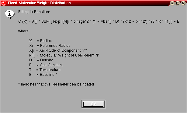
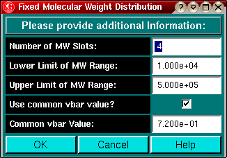
4. Fixed Molecular Weight Distribution: In this model, the molecular weights are preset as an evenly divided distribution of molecular weights between some lower and upper molecular weight limit. This model can be used for any experiment, since it fits the experiment in an almost model-independent way. Several diagnostic plots are provided with this model to ascertain what nonlinear model may be most appropriate for fitting. Fitting with this model can prove helpful for cases where you need to distinguish between self-associating and noninteracting systems.

   A predetermined molecular weight distribution with the molecular weight parameter kept fixed is used to fit all scans independently with general least squares. Since no exponents are fitted, the fitting function can be considered a linear combination of nonlinear terms, which is linear in the coefficients that are fitted. The coefficients are nothing more than the amplitudes for each exponential term with a different fixed molecular weight. Use at least 3 different molecular weight terms to describe a model-independent system.

   If the residuals for this fit do not come out perfectly random and show systematic drift, the molecular weight distribution is not set up correctly. Perform a single component, ideal fit first, and repeat the fixed molecular weight distribution model by centering your molecular weight distribution around the molecular weight obtained by the single component fit.

   After the fit completes with satisfactory residuals, you can display the results in one of three ways:

   • ln(C) vs. r²: Plots the log of the concentration of each fit versus the square of the radius. If multiple components are present in appreciable amounts, the plots will not be linear. The example shown here reflects a self-associating monomer-dimer system.

   • MW vs. r²: Plots the molecular weight for each fit at each point versus the square of the radius. If the plots roughly overlay, the sample is most likely non-interacting. If the plots follow roughly the sample profile, but each plot at a different position, the sample is most likely self-associating. If the plots have multiple inflection points, multiple species are probably present. The example shown reflects the same self-associating monomer-dimer model as shown above.

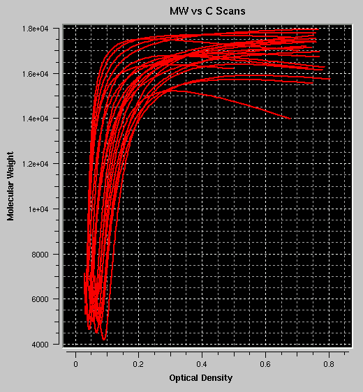
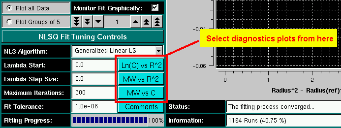
   • MW vs. C: Plots the molecular weight for each fit at each point versus the concentration at that point. If the plots roughly overlay, the sample is most likely following a concentration dependent self-association process. If the plots follow roughly the sample profile, but each plot at a different position, the sample is most likely non-interacting and heterogeneous in composition. If the plots have multiple inflection points, multiple species are probably present. The example shown reflects the same self-associating monomer-dimer model as shown above.

   The plotting functions listed above are available for this model only and can be accessed from the fitting control panel.

   The following parameters are fitted:

   • The amplitudes for each molecular weight term for each included scan (local)
   • The baseline (or zeroth order term) for each included scan (local)

   The following parameters are fixed:

   • Each molecular weight term (global)

   The model number for this model is "3".

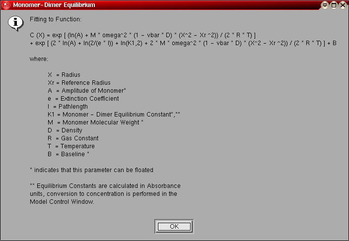
5. Monomer-Dimer Equilibrium: This model can be used to fit an ideal, reversibly self-associating monomer-dimer system. The following parameters are fitted:
   • The monomer molecular weight (global)
   • The log of the amplitude of the monomer molecular weight term for each included scan (local)
   • The log of the monomer-dimer association constant (global)
   • The baseline for each included scan (local)

   The model number for this model is "4".

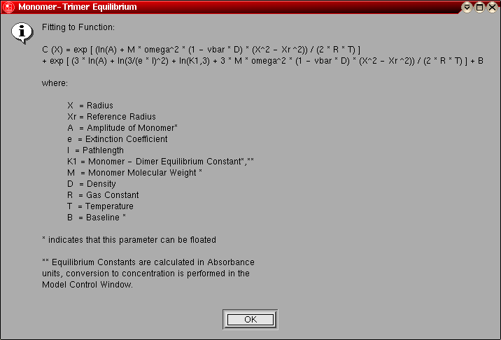
6. Monomer-Trimer Equilibrium: This model is identical to the monomer-dimer equilibrium model, except instead of a dimer the association is for a trimer.

   The model number for this model is "5".

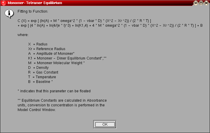
7. Monomer-Tetramer Equilibrium: This model is identical to the monomer-dimer equilibrium model, except instead of a dimer the association is for a tetramer.

   The model number for this model is "6".

8. Monomer-Pentamer Equilibrium: This model is identical to the monomer-dimer equilibrium model, except instead of a dimer the association is for a pentamer.

   The model number for this model is "7".

9. Monomer-Hexamer Equilibrium: This model is identical to the monomer-dimer equilibrium model, except instead of a dimer the association is for a hexamer.

   The model number for this model is "8".

10. Monomer-Heptamer Equilibrium: This model is identical to the monomer-dimer equilibrium model, except instead of a dimer the association is for a heptamer.

    The model number for this model is "9".

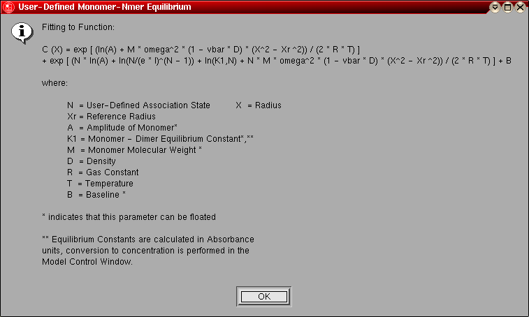
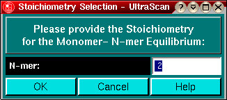
11. User-defined Monomer-Nmer Equilibrium: This model is identical to the monomer-dimer equilibrium model, except instead of a dimer the association is for a user-defined stoichiometry. You can define your desired stoichiometry in the monomer-Nmer stoichiometry selection panel.

    The model number for this model is "10".

12. Monomer-Dimer-Trimer Equilibrium: This model can be used to fit an ideal, reversibly self-associating monomer-dimer-trimer system. The following parameters are fitted:
    • The monomer molecular weight (global)
    • The log of the amplitude of the monomer molecular weight term for each included scan (local)
    • The log of the monomer-dimer association constant (global)
    • The log of the monomer-trimer association constant (global)
    • The baseline for each included scan (local)

    The model number for this model is "11".

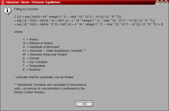
13. Monomer-Dimer-Tetramer Equilibrium: This model can be used to fit an ideal, reversibly self-associating monomer-dimer-tetramer system. The following parameters are fitted:
    • The monomer molecular weight (global)
    • The log of the amplitude of the monomer molecular weight term for each included scan (local)
    • The log of the monomer-dimer association constant (global)
    • The log of the monomer-tetramer association constant (global)
    • The baseline for each included scan (local)

    The model number for this model is "12".

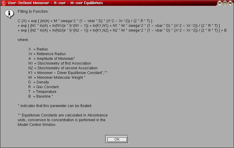
14. User-defined Monomer - N-mer - M-mer Equilibrium: This model can be used to fit an ideal, reversibly self-associating monomer - N-mer - M-mer system. You can define the stoichiometries for the N and M associations using the stoichiometry selection panel. The following parameters are fitted:
    • The monomer molecular weight (global)
    • The log of the amplitude of the monomer molecular weight term for each included scan (local)
    • The log of the monomer - N-mer association constant (global)
    • The log of the monomer - M-mer association constant (global)
    • The baseline for each included scan (local)

    The model number for this model is "13".

Previous: Fitting Information

Model-Specific Information