Manual

Combining C(s) distributions:

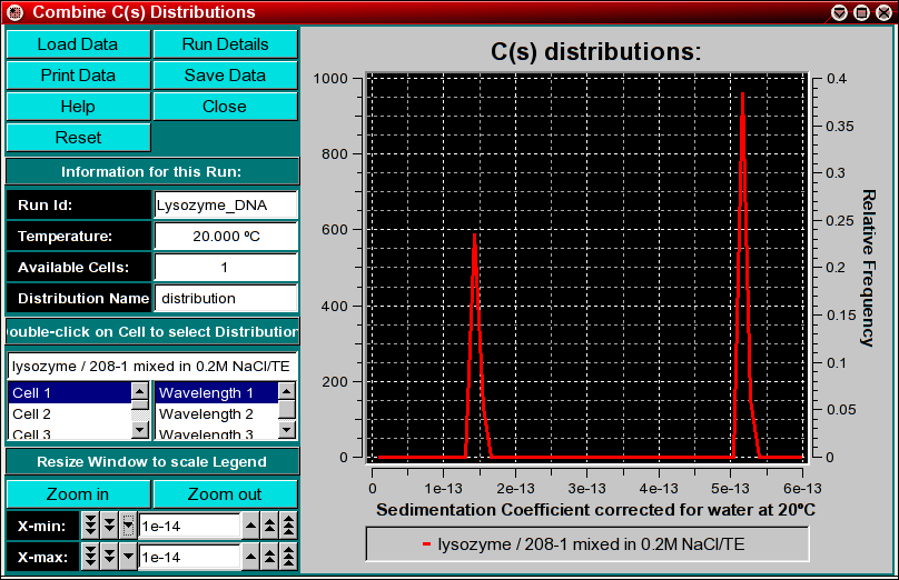
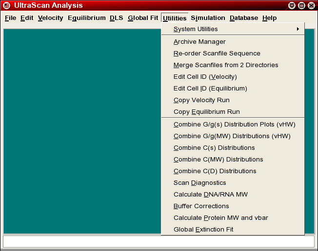
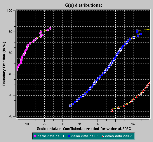
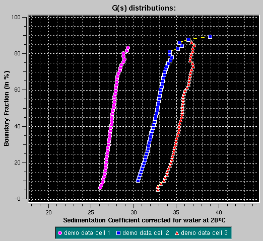
This program enables you to combine multiple sedimentation coefficient distributions from the C(s) analysis into a single plot. You can combine multiple datasets (either from different cells of the same run or from different runs) by using the "Combine C(s) Distributions" item from the Utilities menu. This will allow you to compare molecular weight distributions (which are derived from integral distributions) from different runs and different cells to each other. This may be useful if you analyzed the same sample under different conditions, for example, different pH levels or different concentrations. If the samples are the same, the distributions should overlay, if the samples behave differently, the distributions will be shifted against each other.

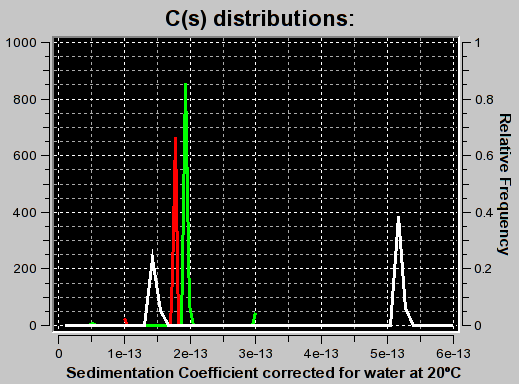
Important Note: The C(s) analysis can produce misleading results and artifactual peaks under certain conditions. If the f/f0 ratio is overestimated, additional artifactual peaks can occur.

Example:

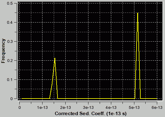	f/f0=1.2 (appropriate for first peak and corresponding to the true C(s) distribution as verfified by van Holde - Weischet and finite element analysis)
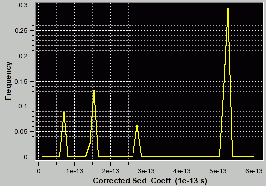	f/f0=3.1 (appropriate for second peak)
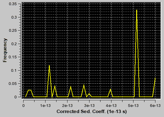	f/f0=3.1 (appropriate for second peak)

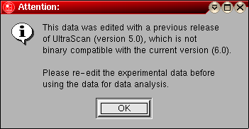
Important Note: In addition to uncertainties about multiple peaks in the distribution, there is another problem users of the C(s) analysis need to be aware of: The molecular weight and diffusion coefficient distributions generated by the C(s) method are based on a single f/f0 value either set or fitted in the C(s) analysis, and on a single vbar value identified with this run. If either the vbar or the f/f0 value is incorrect, the molecular weight and diffusion coefficient distributions will also be incorrect. In general, it is unlikely that multiple components in a single experiment will have the same f/f0 value. This unlikelyhood is translated into the reliability of these distribution. If only a single component is visible in the distribution it is more likely that the value determined for f/f0 is correct.

You can remove erroneously added distributions by double clicking on the distribution to remove it. The curve will be highlighted in white and a message window will ask you if you want to delete it. Confirm or cancel.

Explanation for fields and buttons:

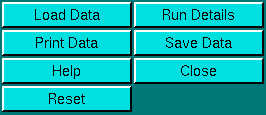Click on these buttons to control the van Holde - Weischet analysis. Load Data: Load edited data sets (with the *.us suffix). A file dialogue will allow you to select a previously edited and saved velocity experiment. If the data was edited with a version of UltraScan less than the current version, an error message will be displayed. Run Details: View the diagnostic details for a particular run. Print Data: Load the printer control panel for printing of plot graphics Save Data: Write out a copy of all distributiones to an ASCII formatted data file suitable for import into a spreadsheet plotting program. The data will be saved in a file called "cofs_distrib.dat" in your results directory (see configuration panel). See "File Structures and Formats" for details. The descriptions in the legend for each dataset is saved in an ASCII file called "cofs_distrib.txt". Note: These files are overwritten each time this button is clicked. Only the last version of the analysis will be saved! You can associate the distribution file by giving it the same name as the run to whose report you would like to add the distribution information. Then the data will be saved in the report directory with the name of the run. This way you can avoid overwriting distribution files. Help: This help file Close: Close the "Combine C(s) Distribution" window. Reset: Reset the plot window and delete all distributions and the legend. After clicking on "Reset" you can start with a new, empty plot window.

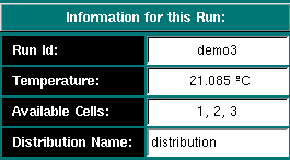
Run Information:

Run ID: The name of the run given during editing Temperature: The average temperature calculated from the entire run Available Cells: The numbers the cells that contain analyzable data Distribution Name: The name under which the html report will be saved. If you make this name the same as the dataset, the combined distribution data will be included in the html report for that dataset. If the default name "distribution" is left unchanged, a separate directory called "distribution" will be created under the html report directory. For more information on the html reports, please see the html report manual page.

Experimental Parameters:

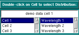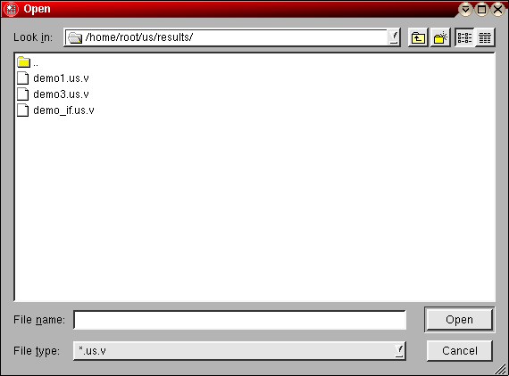
Single-clicking on a cell or wavelength will bring up the sample description of that cell and wavelength. If no data is available for your selection, it will be indicated in the top field. Double-clicking on a valid selection will add the integral distribution of that selection to the plot area and add an item to the legend. Scroll through this list to bring up information for cells > 3. 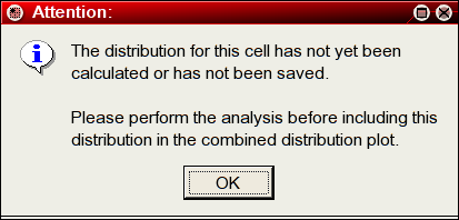If you double-click on an invalid item, an error message window will appear. If the selection is valid, but a distribution plot has not been saved from the van Holde - Weischet analysis, an error message will appear. If you decide to eliminate a distribution plot from the combined overlay, simply click on the scan to be removed in the plot area, and you will be asked if you want to delete the highlighted scan. The scan about to be deleted will be highlighted in white.

Analysis Controls:

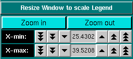Sometimes the legend does not appear correctly resized (for example, if the item in the description of the sample is too long for the provided screen area), In that case, it is necessary to resize the window to a larger size to accommodate the longer text. Click on "Zoom in" or "Zoom out" to present a smaller or larger scale of the item. Clicking on the X-min and X-max counters allows you to manually set the X-min/max limits of the data plot.